🧬 R语言时间序列蛋白质组学聚类分析完整教程
在蛋白质组学研究中,时间序列分析是理解蛋白质动态变化模式的重要方法。本文将详细介绍如何使用R语言的TCseq包进行时间序列蛋白质组学聚类分析。
🎯 分析目标
通过时间序列聚类分析,我们可以:
- 📈 识别蛋白质在不同时间点的表达模式
- 🔍 发现具有相似变化趋势的蛋白质群组
- 📊 可视化蛋白质动态变化规律
- 🧩 为后续功能富集分析提供基础
📦 所需R包
1
2
3
4
5
6
7
8
9
10
11
12
|
library(TCseq)
library(readxl)
library(pheatmap)
library(dplyr)
library(ggplot2)
library(gridExtra)
library(patchwork)
|
⚙️ 参数配置
🔧 基本参数设置
1
2
3
4
5
6
7
8
9
10
11
12
13
14
15
16
17
18
19
20
21
22
23
24
|
work_dir <- "~/mice33/work/lab/深圳三院250730"
setwd(work_dir)
input_file <- "2. 数据结果/2. 差异统计/1. 蛋白定量统计.xlsx"
sheet_name <- "蛋白定量统计"
cluster_num <- 6
random_seed <- 123
algo_method <- 'cm'
time_points <- list(
T1 = c("A1", "A2", "A3"),
T2 = c("B1", "B2", "B3"),
T3 = c("C1", "C2", "C3"),
T4 = c("D1", "D2", "D3")
)
|
🎨 可视化参数
1
2
3
4
5
6
|
figure_width <- 15
figure_height <- 10
single_plot_width <- 8
single_plot_height <- 6
language <- "EN"
|
📊 数据读取与预处理
📁 数据读取函数
1
2
3
4
5
6
7
8
9
10
11
12
13
14
15
16
17
18
19
20
21
22
23
24
25
26
27
28
29
30
31
32
33
34
35
| read_and_process_data <- function(file_path, sheet_name, time_points) {
cat("正在读取数据...\n")
if (!file.exists(file_path)) {
stop("输入文件不存在:", file_path)
}
protein_data <- read_excel(file_path, sheet = sheet_name)
abundance_cols <- grep("Abundances.*Normalized", colnames(protein_data), value = TRUE)
if (length(abundance_cols) == 0) {
abundance_cols <- grep("Abundance", colnames(protein_data), value = TRUE)
}
sample_matrix <- as.matrix(protein_data[, abundance_cols, drop = FALSE])
if ("Gene Symbol" %in% colnames(protein_data)) {
rownames(sample_matrix) <- make.unique(protein_data$`Gene Symbol`)
} else if ("Protein" %in% colnames(protein_data)) {
rownames(sample_matrix) <- make.unique(protein_data$Protein)
} else {
rownames(sample_matrix) <- paste0("Protein_", 1:nrow(sample_matrix))
}
colnames(sample_matrix) <- gsub(".*:", "", colnames(sample_matrix))
colnames(sample_matrix) <- trimws(colnames(sample_matrix))
return(sample_matrix)
}
|
📈 时间点均值计算
1
2
3
4
5
6
7
8
9
10
11
12
13
14
15
16
17
18
19
20
21
22
23
| calculate_timepoint_means <- function(sample_matrix, time_points) {
cat("计算时间点均值...\n")
mean_list <- list()
for (i in seq_along(time_points)) {
tp_name <- names(time_points)[i]
tp_samples <- time_points[[i]]
available_samples <- intersect(tp_samples, colnames(sample_matrix))
if (length(available_samples) == 0) {
stop("时间点", tp_name, "的样本在数据中未找到")
}
mean_list[[tp_name]] <- rowMeans(sample_matrix[, available_samples, drop = FALSE], na.rm = TRUE)
cat("时间点", tp_name, "使用", length(available_samples), "个样本\n")
}
mean_matrix <- do.call(cbind, mean_list)
colnames(mean_matrix) <- names(time_points)
return(mean_matrix)
}
|
🧹 数据预处理
1
2
3
4
5
6
7
8
9
10
11
12
13
14
15
16
| preprocess_data <- function(mean_matrix) {
cat("数据预处理...\n")
cat("缺失值数量:", sum(is.na(mean_matrix)), "\n")
cat("零值数量:", sum(mean_matrix == 0, na.rm = TRUE), "\n")
complete_rows <- complete.cases(mean_matrix)
mean_matrix_clean <- mean_matrix[complete_rows, ]
mean_matrix_log <- log2(mean_matrix_clean + 1)
return(list(clean = mean_matrix_clean, log = mean_matrix_log))
}
|
🎯 聚类分析
📊 TCseq聚类分析
1
2
3
4
5
6
7
8
9
10
11
12
13
| perform_clustering <- function(data_matrix, k = 6, algorithm = 'cm', seed = 123) {
cat("开始聚类分析...\n")
set.seed(seed)
tcseq_result <- timeclust(data_matrix,
algo = algorithm,
k = k,
standardize = TRUE)
return(tcseq_result)
}
|
🔍 聚类算法说明
| 算法类型 |
代码 |
特点 |
适用场景 |
| 模糊C均值 |
'cm' |
允许软聚类,蛋白质可属于多个类别 |
推荐,适合生物数据 |
| K均值 |
'km' |
硬聚类,每个蛋白质只属于一个类别 |
快速,适合大数据 |
| 层次聚类 |
'hc' |
基于距离的聚类方法 |
适合探索性分析 |
📈 结果可视化
🎨 时间序列图
1
2
3
4
5
6
7
8
9
10
11
12
13
14
15
16
17
18
19
20
21
22
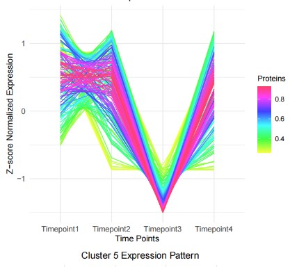
| create_timeseries_plots <- function(tcseq_result, language = "EN") {
cat("创建时间序列图...\n")
p <- timeclustplot(tcseq_result,
value = 'z-score',
cols = 3,
axis.line.size = 0.8,
title.size = 12)
cluster_counts <- table(tcseq_result@cluster)
for(i in 1:length(p)) {
p[[i]] <- p[[i]] +
labs(title = paste("Cluster", i, "(n =", cluster_counts[i], ")"),
x = "Time Points",
y = "Z-score Normalized Expression") +
theme_minimal()
}
return(p)
}
|
🔥 聚类中心热图
1
2
3
4
5
6
7
8
9
10
11
12
13
14
15
16
17
18
19
20
21
22
23
| create_heatmap <- function(tcseq_result, language = "EN") {
cluster_counts <- table(tcseq_result@cluster)
heatmap_data <- tcseq_result@centers
rownames(heatmap_data) <- paste0("Cluster ", 1:nrow(heatmap_data),
"\n(n=", cluster_counts, ")")
colnames(heatmap_data) <- paste("Time Point", 1:ncol(heatmap_data))
heatmap_plot <- pheatmap(heatmap_data,
cluster_rows = FALSE,
cluster_cols = FALSE,
display_numbers = TRUE,
number_format = "%.2f",
main = "Time-series Expression Patterns (Z-score)",
color = colorRampPalette(c("blue", "white", "red"))(50),
cellwidth = 35,
cellheight = 35,
silent = TRUE)
return(list(plot = heatmap_plot, data = heatmap_data))
}
|
📊 综合折线图
1
2
3
4
5
6
7
8
9
10
11
12
13
14
15
16
17
18
19
20
21
22
23
24
25
26
27
28
29
30
31
32
33
34
35
| create_comprehensive_plot <- function(tcseq_result, language = "EN") {
cluster_counts <- table(tcseq_result@cluster)
cluster_centers_df <- data.frame(
Cluster = factor(rep(1:nrow(tcseq_result@centers), each = ncol(tcseq_result@centers))),
TimePoint = rep(1:ncol(tcseq_result@centers), nrow(tcseq_result@centers)),
Expression = as.vector(t(tcseq_result@centers)),
Count = rep(cluster_counts, each = ncol(tcseq_result@centers))
)
cluster_centers_df$Cluster_Label <- paste0("Cluster ", cluster_centers_df$Cluster,
" (n=", cluster_centers_df$Count, ")")
comprehensive_plot <- ggplot(cluster_centers_df,
aes(x = TimePoint, y = Expression,
color = Cluster_Label,
group = Cluster_Label)) +
geom_line(size = 1.2, alpha = 0.8) +
geom_point(size = 3, alpha = 0.9) +
scale_x_continuous(breaks = 1:max(cluster_centers_df$TimePoint),
labels = paste("Time Point", 1:max(cluster_centers_df$TimePoint))) +
labs(title = "Time-series Expression Patterns of All Clusters",
subtitle = "Based on Fuzzy C-means Clustering",
x = "Time Points",
y = "Z-score Normalized Expression",
color = "Clusters") +
theme_minimal() +
theme(plot.title = element_text(size = 14, hjust = 0.5, face = "bold"),
plot.subtitle = element_text(size = 12, hjust = 0.5)) +
scale_color_brewer(type = "qual", palette = "Set2")
return(comprehensive_plot)
}
|
📁 结果整理与保存
📊 结果数据整理
1
2
3
4
5
6
7
8
9
10
11
12
13
14
15
16
17
18
19
20
21
22
23
24
25
26
27
28
29
30
31
32
33
34
35
| organize_results <- function(tcseq_result, data_clean, data_log, language = "EN") {
protein_names <- rownames(data_log)
cluster_assignments <- tcseq_result@cluster
cluster_counts <- table(cluster_assignments)
cluster_results <- data.frame(
Protein = protein_names,
Cluster = cluster_assignments,
stringsAsFactors = FALSE
)
for (i in 1:ncol(data_log)) {
cluster_results[paste0("Timepoint", i, "_zscore")] <- data_log[, i]
}
for (i in 1:ncol(data_clean)) {
cluster_results[paste0("Timepoint", i, "_original")] <- data_clean[, i]
}
cluster_summary <- data.frame(
Cluster = 1:nrow(tcseq_result@centers),
Count = as.numeric(cluster_counts)
)
for (i in 1:ncol(tcseq_result@centers)) {
cluster_summary[paste0("T", i, "_Center")] <- round(tcseq_result@centers[, i], 3)
}
return(list(results = cluster_results, summary = cluster_summary))
}
|
💾 批量保存结果
1
2
3
4
5
6
7
8
9
10
11
12
13
14
15
16
17
18
19
20
21
22
23
24
25
26
27
28
29
30
31
32
33
34
| save_all_results <- function(tcseq_result, organized_results, plots, heatmap_info,
comprehensive_plot, integrated_plot, results_dir) {
if (!dir.exists(results_dir)) {
dir.create(results_dir)
}
write.csv(organized_results$results,
file.path(results_dir, "Complete_Clustering_Results.csv"),
row.names = FALSE)
write.csv(organized_results$summary,
file.path(results_dir, "Cluster_Pattern_Summary.csv"),
row.names = FALSE)
cluster_counts <- table(tcseq_result@cluster)
for(i in 1:length(cluster_counts)) {
cluster_proteins <- organized_results$results[organized_results$results$Cluster == i, ]
write.csv(cluster_proteins,
file.path(results_dir, paste0("Cluster_", i, "_proteins.csv")),
row.names = FALSE)
}
ggsave(file.path(results_dir, "Comprehensive_Line_Plot.pdf"),
plot = comprehensive_plot, width = 12, height = 8)
pdf(file.path(results_dir, "Cluster_Centers_Heatmap.pdf"), width = 10, height = 8)
print(heatmap_info$plot)
dev.off()
}
|
🚀 完整执行流程
🔄 主程序函数
1
2
3
4
5
6
7
8
9
10
11
12
13
14
15
16
17
18
19
20
21
22
23
24
25
26
27
28
29
30
31
32
33
34
35
36
| main_analysis <- function() {
cat("开始时间序列蛋白质组学聚类分析...\n")
sample_matrix <- read_and_process_data(input_file, sheet_name, time_points)
mean_matrix <- calculate_timepoint_means(sample_matrix, time_points)
processed_data <- preprocess_data(mean_matrix)
tcseq_result <- perform_clustering(processed_data$log, cluster_num, algo_method, random_seed)
plots <- create_timeseries_plots(tcseq_result, language)
heatmap_info <- create_heatmap(tcseq_result, language)
comprehensive_plot <- create_comprehensive_plot(tcseq_result, language)
organized_results <- organize_results(tcseq_result, processed_data$clean, processed_data$log)
save_all_results(tcseq_result, organized_results, plots, heatmap_info,
comprehensive_plot, integrated_plot, results_dir)
print_summary(organized_results, tcseq_result)
return(list(
tcseq_result = tcseq_result,
organized_results = organized_results,
plots = plots,
comprehensive_plot = comprehensive_plot
))
}
results <- main_analysis()
|
📊 结果解读
🔍 聚类模式识别
分析完成后,通常会得到以下几种典型的时间序列模式:
- 📈 上升型:蛋白质表达量随时间逐渐增加
- 📉 下降型:蛋白质表达量随时间逐渐减少
- 🔺 早期峰型:在早期时间点达到最高表达
- 🔻 晚期峰型:在晚期时间点达到最高表达
- 📊 稳定型:表达量在时间序列中保持相对稳定
- 🌊 波动型:表达量呈现周期性变化
📈 生物学意义
不同的聚类模式可能反映:
- 早期应答基因:快速响应刺激的蛋白质
- 晚期应答基因:延迟响应的调节蛋白质
- 持续表达基因:维持细胞基本功能的蛋白质
- 周期性调节基因:参与细胞周期调控的蛋白质
🎯 使用建议
✨ 参数优化
聚类数量选择:
1
2
3
4
5
|
for(k in 4:8) {
result_k <- timeclust(data_matrix, k = k)
}
|
算法选择:
1
2
3
4
5
|
algorithms <- c('cm', 'km', 'hc')
results_compare <- lapply(algorithms, function(alg) {
timeclust(data_matrix, algo = alg, k = 6)
})
|
📋 质量控制
- 检查输入数据的质量和完整性
- 确保样本分组信息正确
- 验证聚类结果的生物学合理性
- 进行功能富集分析验证聚类结果
🔗 扩展分析
🧬 功能富集分析
1
2
3
4
5
6
7
8
9
10
11
12
13
|
library(clusterProfiler)
for(i in 1:cluster_num) {
cluster_genes <- organized_results$results[
organized_results$results$Cluster == i, "Protein"
]
go_result <- enrichGO(gene = cluster_genes,
OrgDb = org.Hs.eg.db,
ont = "BP")
}
|
📊 共表达网络分析
1
2
3
4
5
6
7
8
|
library(WGCNA)
cor_matrix <- cor(t(processed_data$log))
|
📚 相关资源
- TCseq包文档:Bioconductor TCseq
- 时间序列分析理论:《Time Series Analysis and Its Applications》
- 蛋白质组学数据分析:《Computational Proteomics》